How to Easily Make a Drop Down List in Excel Like a Pro

Creating a drop down list in Excel allows you to present a list of pre-defined options that users can choose from when entering data.

This prevents errors from users entering invalid values and also standardizes the data being entered. Excel drop downs make data entry much easier.

In this comprehensive guide, you’ll learn multiple methods to create different types of drop downs in Excel.

Intro to Excel Drop Down Lists

A drop down list contains a predefined set of values that appears as a drop down menu for easy selection.

Here are some key points about Excel drop downs:

• They simplify data entry and prevent invalid entries
• You can create them manually or link them to a cell range
• Items can be selected from the drop down or directly typed in the cell
• Useful for standardizing data in things like categories, statuses, etc.

In the steps below, you’ll learn how to create all kinds of useful drop downs for your Excel workbooks.

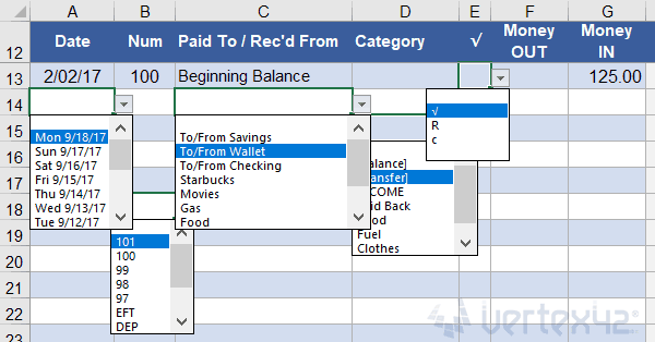
Method 1: Manually Create a Drop Down List

The easiest way to make a dropdown in Excel is by manually typing the items. Here are the steps:

1. Select the cell where you want to put the drop down
2. Under the Data tab ribbon, click Data Validation
3. In the Data Validation window, set:Allow: as List
4. For Source enter your list items separated by commas
5. Click OK

This creates a manual list dropdown in the selected cell.

You can directly type values into the cell with the dropdown instead of selecting from the list.

This works good for short, static lists.

Pro Tip: You can reference cell ranges as the Source instead of typing values manually to reuse dropdowns.

Let’s look at more robust ways to create dynamic dropdowns.

Method 2: Link Drop Down List to a Cell Range

Hard-coding dropdown items isn’t the best practice. It’s better to link to a cell range.

This way you can add, remove or edit items in one place and the dropdown updates automatically everywhere that range is used.

Follow below steps to do this:

1. Enter list items into a worksheet cell range
2. Select the dropdown cell, Go to Data > Data Validation
3. Set Allow: as List
4. For the Source field, enter the cell range reference that contains your list
5. Press OK

Now the dropdown is dynamically linked to your list range.

When you add/remove items from the list range, the dropdown updates automatically!

Method 3: Create a Dynamic Named Range for Dropdown

Directly referencing a cell range works but isn’t the cleanest approach.

An even better way is to use a dynamic named range.

Here are the steps to do that:

1. Select the list cell range
2. Go to Formulas > Define Name
3. Name the range, Eg. “CategoryList”
4. Select cell for dropdown, Go to Data > Data Validation
5. Set Allow: as List
6. For Source enter the named range, Eg. CategoryList
7. Press OK

This uses Excel named ranges to create dropdown list.

The benefit is – you only need to update the named range when you modify list items instead of all validations that refer this list. Making edits simpler.

Also this approach leads to cleaner code that is easier to interpret and manage vs direct cell references.

Method 4: Create Cascading Dropdown Lists in Excel

What if you want dropdowns that dynamically filter based on previous selections?

This can be achieved by cascading dropdown lists in Excel.

For example – Region > Country > City selections that display only relevant values.

Here are the steps to create them:

1. Set up named ranges for each dropdown list, E.g. Regions, Countries, Cities
2. Create first dropdown by linking the named range to cell data validation
3. Cell links to second dropdown uses a formula like:
   =OFFSET(Countries,MATCH([FirstSelection],Regions,0),0)
4. Similarly cell links to third dropdown will be: =OFFSET(Cities,MATCH([SecondSelection],Countries,0),0)

This sets up dropdowns that cascade based on selections in previous dropdowns.

It works by matching the previous selection value and getting only relevant items for next dropdown.

Pretty neat! Play around with such formulas to create multi-level cascading dropdowns.

Useful Examples of Excel Drop Down Lists

Here are some good examples of using dropdown lists:

• Categories
  • Product, article and other categories
• Statuses
  • Order statuses, deal stages, pipeline steps etc
• Classifications
  • Groups, types and other classifications
• Selection Lists
  • Country, region, city, store etc lists
• Ratings
  • 1 to 5 rating, performance levels
• Standard Values
  • Gender, salary range, etc fixed lists
• Navigation
  • Links, prompts and navigation options

I’m sure you can think of several more!

Excel dropdown lists give you an easy way to standardize data and simplify data entry while minimizing errors.

Top 5 Frequently Asked Questions

Here are answers to 5 most frequently asked questions about Excel drop downs:

1. Can I sort a dropdown list in Excel?Yes, you can apply sorting to the source cell range to rearrange items in dropdown. Or sort the named range if you use that approach. Don’t sort data validation cells.
2. Is it possible to make a dropdown list required in Excel?Yes, check the “Ignore blank” option under data validation to make dropdown selection required. Leave it unchecked to allow blank values.
3. Can I add a default value to a dropdown list in Excel?There is no direct way, but you can achieve it with helper cells. First cell has data validation for the dropdown. Second cell checks if first cell is blank and returns the default value. Else it mirrors first cell value. Reference second cell everywhere.
4. Why is my dropdown not showing full list in Excel?Check if cell width is adequate to show the entire dropdown list. Increase column width to always show full dropdown list items without scrolling.
5. How do I get multi-column dropdown lists in Excel?Unfortunately, Excel does not support multi-column dropdown lists natively. VBA macros can be used for this functionality instead of data validation. Or add helper columns.

Hope this helps answer some of the commonly asked questions!

Conclusion

That brings us to the end of this comprehensive guide to creating dropdown lists in Excel.

We looked at a variety of methods:

• Manually entering list items
• Linking dynamic cell ranges
• Using named ranges
• Cascading list options

Dropdown lists will make your spreadsheets more powerful, easier to use, and minimize errors.

Try creating dropdowns in your Excel dashboards and templates. And let me know if you have any questions!